How to Set Up a Thermal Study in SOLIDWORKS Simulation Professional

This guide will go over how to set up a Thermal Study in SOLIDWORKS Simulation Professional. This tutorial will demonstrate two different examples: a steady-state thermal analysis a time-dependent study.

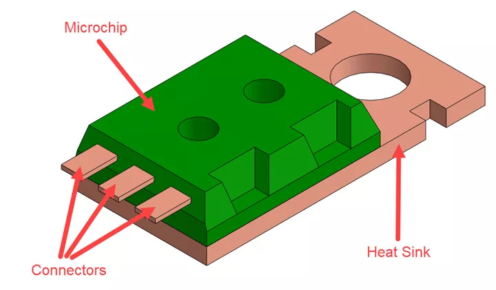
Our model will consist of a few different parts: 

• Microchip – Generating the heat
• Heat Sink – Used to dissipate the heat
• Connectors – Insulated and used to connect to the rest of the electronic components.

Steady-State Thermal Analysis 

For this example, we will be setting it up as a steady-state thermal analysis, which means there is no time factor involved. 

1. We will start by creating a new Thermal Study. 
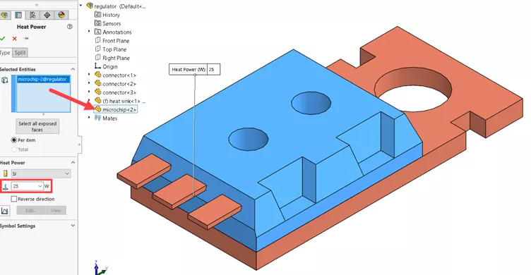
2. Then we are going to define the heat power of the microchip. To do this:
1. Right-click on  Thermal Loads , and select  Heat Power
2. Use the FeatureManager flyout tree to select the microchip part
3. Set the Heat Power to be 25 W
   
   
   
   
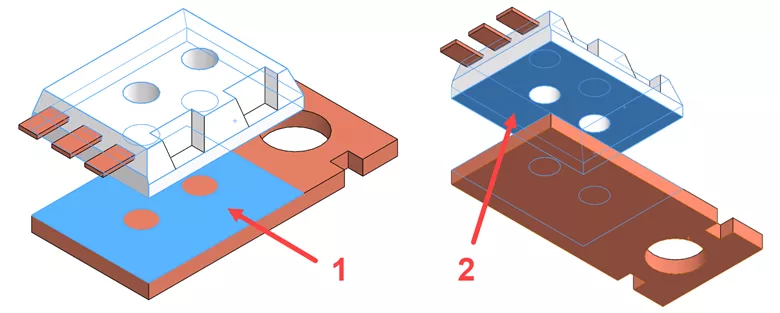
3. Next, we need to consider how this heat is going to be dissipated. Between our microchip and heat sink, we have a thermal conductive glue to help with the dissipation. The glue is not physically modeled, we are going to insert it as a contact resistance. 
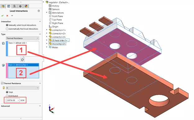
1. Create a  Local Interaction , and make sure it is set to  Thermal Resistance.
2. Click the two faces that touch between the microchip and heat sink. 
1. It can help to explode the assembly.
   
   
   
   
3. Define the contact based on the conductive glue 2.857e-6 K/W
   
   
   
   
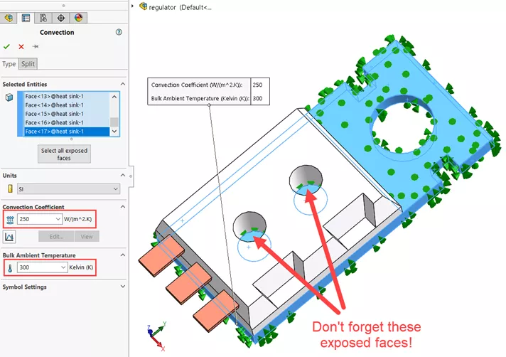
4. We now need to define the convection that is coming off of the rest of the faces on the heat sink. Because the connectors are insulated, we don’t need to define those.  
1. Right-click on  Thermal Loads  and select  Convection.
2. Select all the exposed faces of the heat sink.
3. Define the Convection Coefficient as 250 W/(m^2.K)
4. Define Bulk Ambient Temperature (the temperature that surrounds the model) as 300 Kelvin (K)
   
   
   
   
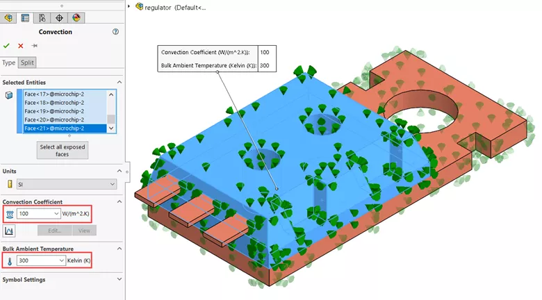
5. Accept that, and start a new Convection for the exposed faces of the microchip.
6. Convection Coefficient is 100 W/(m^2.K), Bulk Ambient Temperature is 300 Kelvin (K).
   
   
   
   
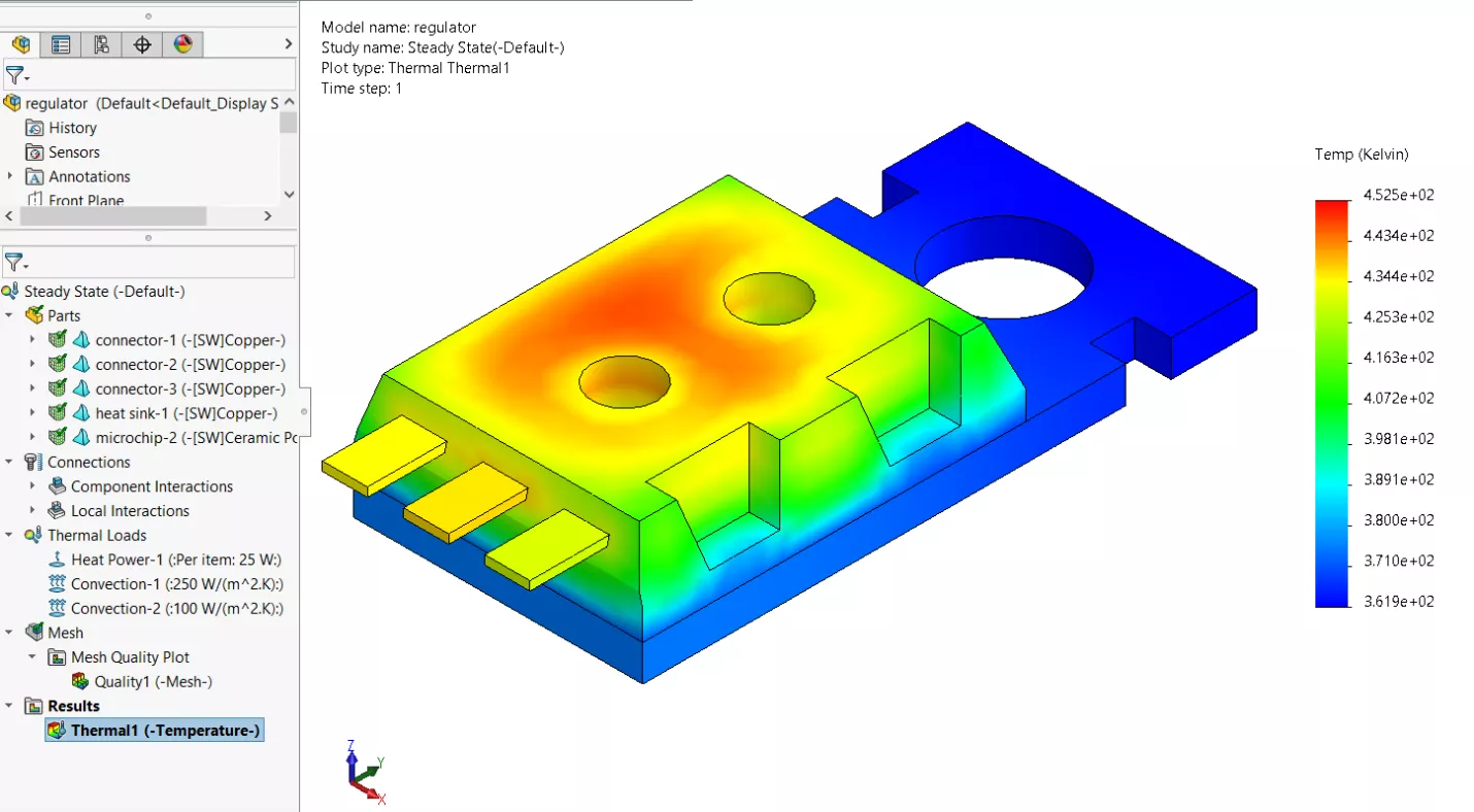
5. We can now run the study and analyze the results. 
   
   
   

Time-Dependent Thermal Analysis 

This example is a time-dependent thermal analysis study, to understand how quickly this will heat and/or cool. (The article Time-based Thermal Stress in SOLIDWORKS Simulation goes into even more detail). We can use the previous setup for this. So, to start, we will copy the Steady-State study. 

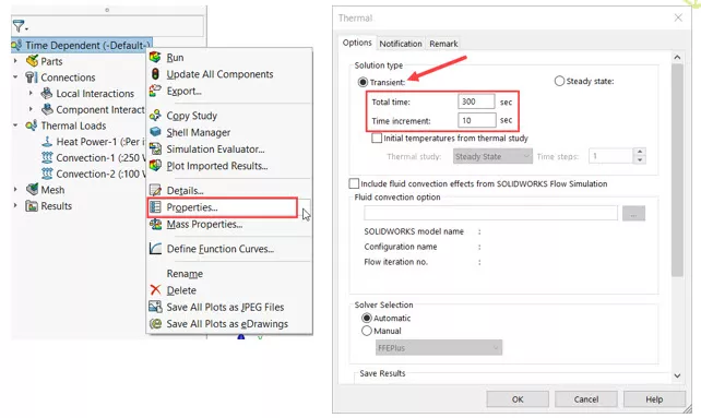
1. In this example, we mainly need to change the properties. To do so:
   1. Right-click on the study name from the tree and select  Properties . 
   2. Under Options, select  Transient  and set the Total time to 300 s, at a time increment of 10 s. 
      
      
      
      
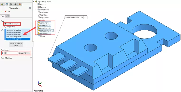
2. The next step is to add an Initial Temperature. To do so:
   1. Right-click on  Thermal Loads  and add a Temperature.
   2. Change it to  Initial Temperature.
   3. Select all the different parts from the FeatureManager fly out tree.
   4. Set the Temperature to be 25 Celcius (ºC).
      
      
      
      
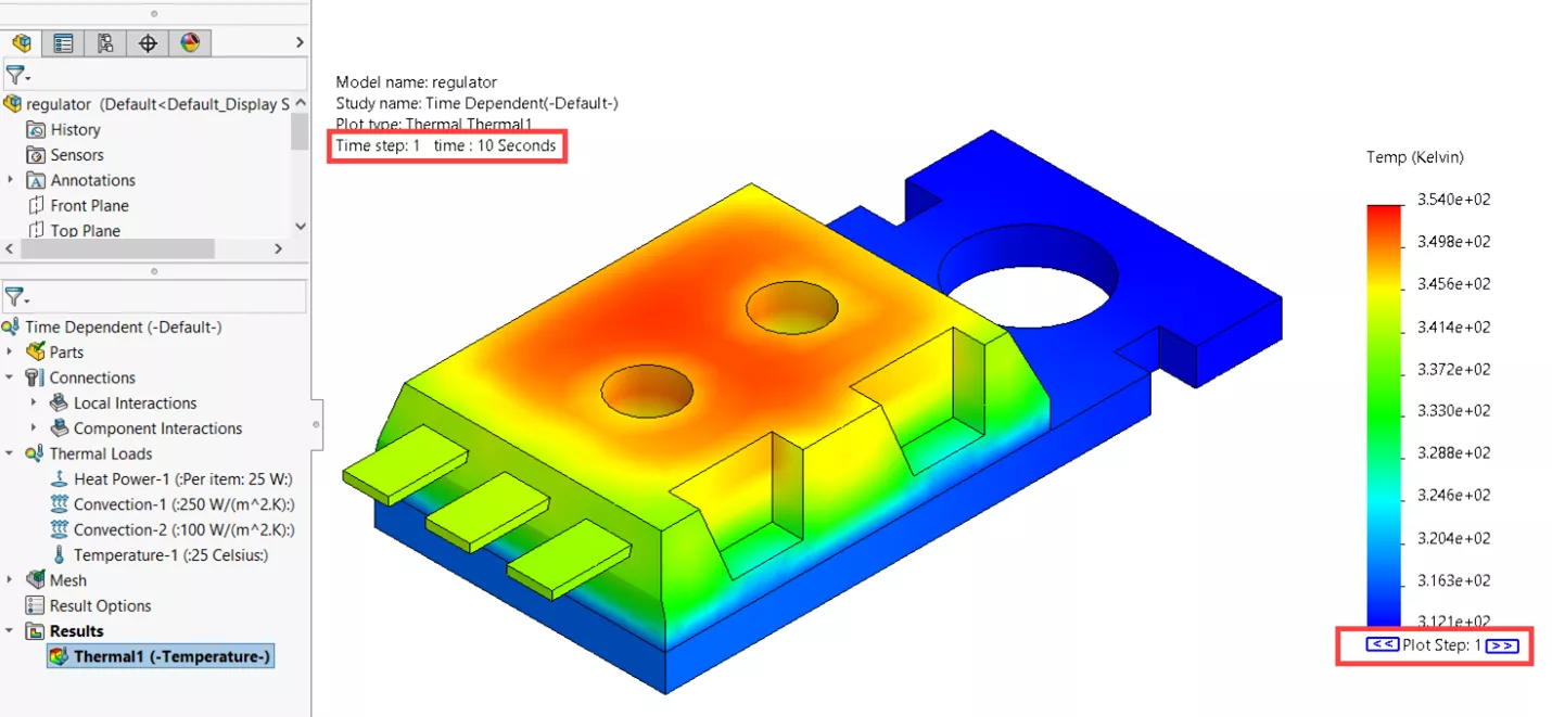
3. Now the study can be ran. The results that initially show, are for Plot Step 1, which is only 10 seconds into the study. 
   
   
   
   
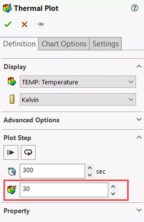
4. To take a look at the results at the different increments:
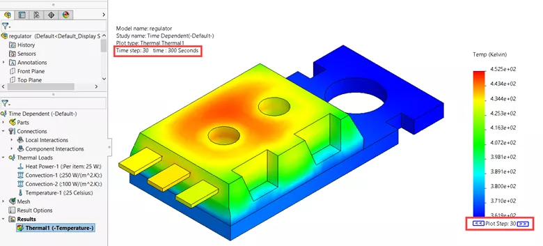
   1. Edit the definition of the Thermal 1  results, and under  Plot Steps,  change the Plot Step to 30, which will show the results after 300 seconds. 
      
      
      
      
      

I hope you found this introduction to Thermal Studies helpful. If you'd like to learn more about SOLIDWORKS Simulation, check out the additional resources below.

More SOLIDWORKS Thermal Study Tutorials

Performing a Thermal Stress Analysis in SOLIDWORKS Simulation (Linear/Nonlinear Static + Flow Simulation)

Using Thermal Boundary Conditions in SOLIDWORKS Simulation to Simulate a Press Fit Connection

  SOLIDWORKS Thermal from Beginning to End 

VIEW ALL SOLIDWORKS SIMULATION TUTORIALS