SOLIDWORKS Flow Simulation Electronics Cooling Part 3: Heat Pipes
Welcome to part 3 of the blog covering the added capability the Electronics Cooling Module offers to SOLIDWORKS Flow Simulation. If you have not done so yet, I recommend reading Part 1 and Part 2. In these previous blogs, we talked about Joule heating, improved PCB definitions, Two Resistor Components and more. This final blog in the series is reserved for the Heat Pipe functionality included in the Electronics Cooling Module.
Heat pipes are a critical component in any modern electronic device. Open up any computer (including some smartphones) and you will probably find a small metal tube traveling from one part of the device to another.
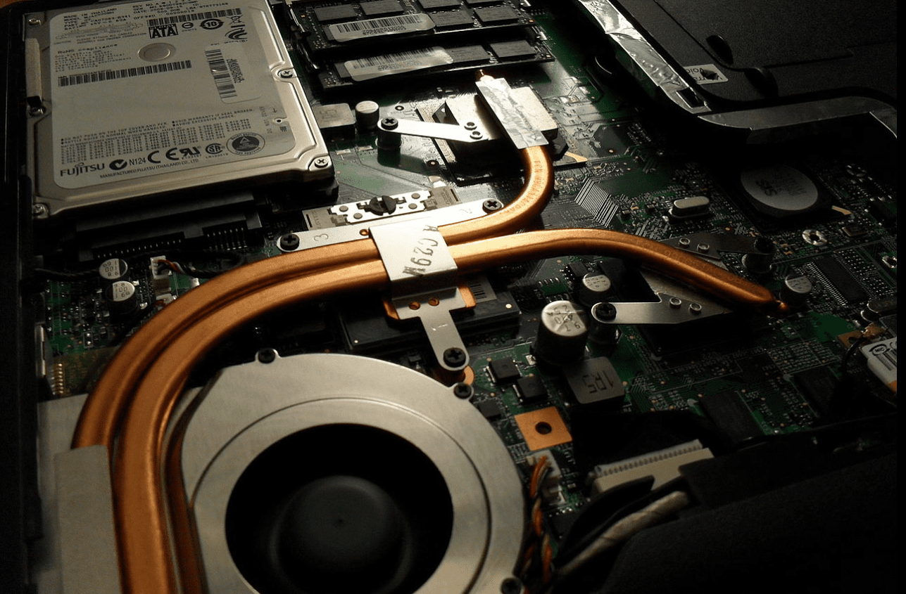
Sample images from http://en.wikipedia.org/wiki/Heat_pipe
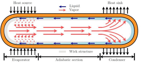
This is a heat pipe, and they are not simply solid metal tubes. Usually, they are hollow, with a wicking material lining the inside to facilitate two-phase cooling. See diagram below from SOLIDWORKS Knowledge Base Article S-063969:
Although Flow Simulation doesn’t support phase transition, this device can be virtually represented with the Electronics Cooling module. It incorporates a mathematical simplification using the effective thermal resistance of the pipe. This is neat because the virtual heat pipe does not even have to be modeled as hollow, a simple solid sweep will do just fine. To define the heat pipe, simply select the component that is to be calculated as the heat pipe. Then select the faces where the heat enters followed by the faces where the heat exits. The last parameter to enter is the effective thermal resistance (if any) of the pipe. See below:
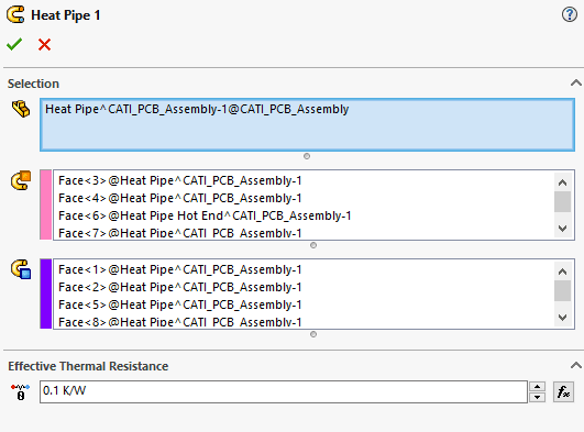
For our application heat is entering the heat pipe from the two-resistor component we defined in the last blog. The exit faces will be on the side of the heat sink I made to finish off the electronics enclosure. I chose an effective thermal resistance of 0.1 K⁰/W for my heat pipe, though real values can be found in data tables online.
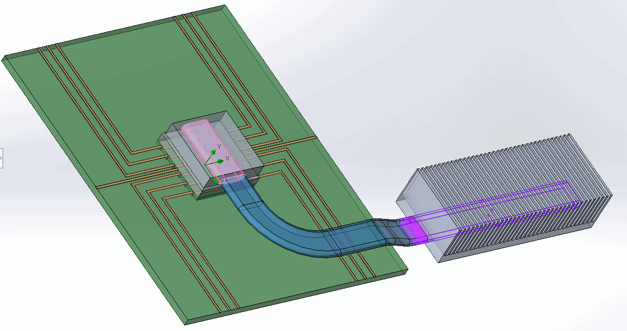
After setting the other parameters necessary to finish the enclosure, the results can be seen below.
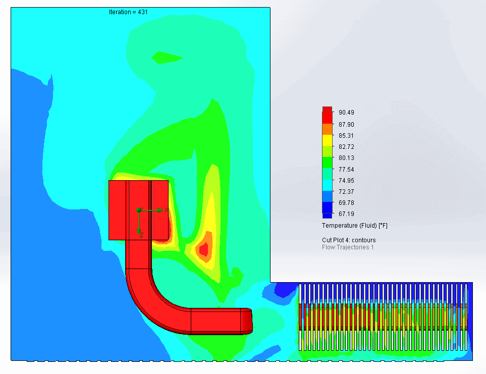
Here you can see that the heat is being pulled away from the chip and distributed at the heat sink on the bottom right. There is an airflow defined by the heat sink that matches the type of fan we would have in the real assembly.
Now to check the temperature of the two-resistor component that is an integral part of this design.
| Temperature Location | Units | Average | Minimum | Maximum |
| Temperature (Junction) | [°F] | 153.48 | 147.64 | 159.53 |
| Temperature (Board) | [°F] | 119.84 | 116.86 | 122.97 |
| Temperature (Case) | [°F] | 104.74 | 98.54 | 111.16 |
So as it turns out, the maximum temperature recorded in the two-resistor component is in the junction, or what I like to think of as the “guts” of the chip. That temperature is 159 degrees Fahrenheit, or about 70 degrees Celsius. This is very typical for a consumer chip at a steady workload.
So finally, the journey through the Electronics Cooling Module of Flow Simulation is done. In Part 1 we covered Joule heating. In Part 2 we covered the creation of the more accurate PCB definition as well as the two-resistor component. Finally, in part 3 we talked about the use of heat pipes in electronics applications. But that’s not all! Also included in the electronics cooling module are expanded libraries in the engineering database specific to electronics applications. There are far too many to list, so if you are interested, please reach out to your local CATI representative today!
Matt Sherak
Applications Engineer, Simulation
Computer Aided Technology, LLC