Tips and Tricks for Post Processing in SOLIDWORKS Simulation

SOLIDWORKS Simulation makes the process of setting up, solving and post-processing a simulation study easy and intuitive. In this blog I will share some of my favorite tips and tricks for the post processing stage.

Tip #1: Start post processing with displacements not stresses

When the SOLIDWORKS Simulation solver is complete, the results are automatically loaded into the results folder. Typically, the results folder will include default plots of von Mises stress, displacement and strain (in that order) and after the run is complete the von Mises stress plot will be highlighted and automatically show on the screen.

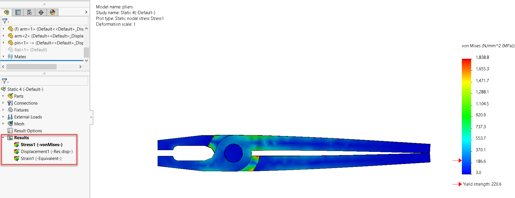
Figure 1: Typical von Mises stress result plot that displays after solution is complete

Since the goal of many simulations is to assess whether and where the part will fail, the temptation is to start diving into the stress results immediately. I strongly recommend against this. Instead, double click on the displacement plot and commence post processing by thoroughly interrogating the deflection and deformation of your part/assembly.

The first thing we often learn from the displacement plot is that there is something wrong with our analysis. Sometimes the stress results look OK, but the displacement plot will show deflections of thousands or even millions of inches or mm! When this happens, we know immediately that something is wrong with our setup. Typically, the part/assembly is not fixtured correctly, or we have not setup our interactions correctly, and hence the results are garbage. In FEA parlance, we have failed to restrain all 6 rigid body modes. In this case there is no need to proceed further with post processing; we must go back to the setup, identify and fix the issue and re-run the analysis.

If we pass the deformation sanity check, the next thing I recommend is to set the deformed shape scale appropriately. In most static simulations, deflections are small relative to the geometry we are analyzing (in fact small deflections are a pre-requisite for a valid linear static analysis). Small deflections are often barely visible to the naked eye, making it hard to visualize where our part/assembly is bending and deflecting. To highlight relative deflections, SOLIDWORKS Simulation can amplify the magnitude of the deformation by applying a scaling factor. Exaggerated deformations are the default plotting option, so be careful; I’ve often heard customers complain that the results don’t look right because the part was bending so much. Remember that the exaggerated deformed shape is just a visual aid to help us identify areas of relatively large deformation. Sometimes a large deformation scale can lead us astray. For example, in my plier analysis if we apply the automatic deformed shape scale (2.98 times exaggeration) the hands of the pliers will pass through each other, which is obviously not possible.

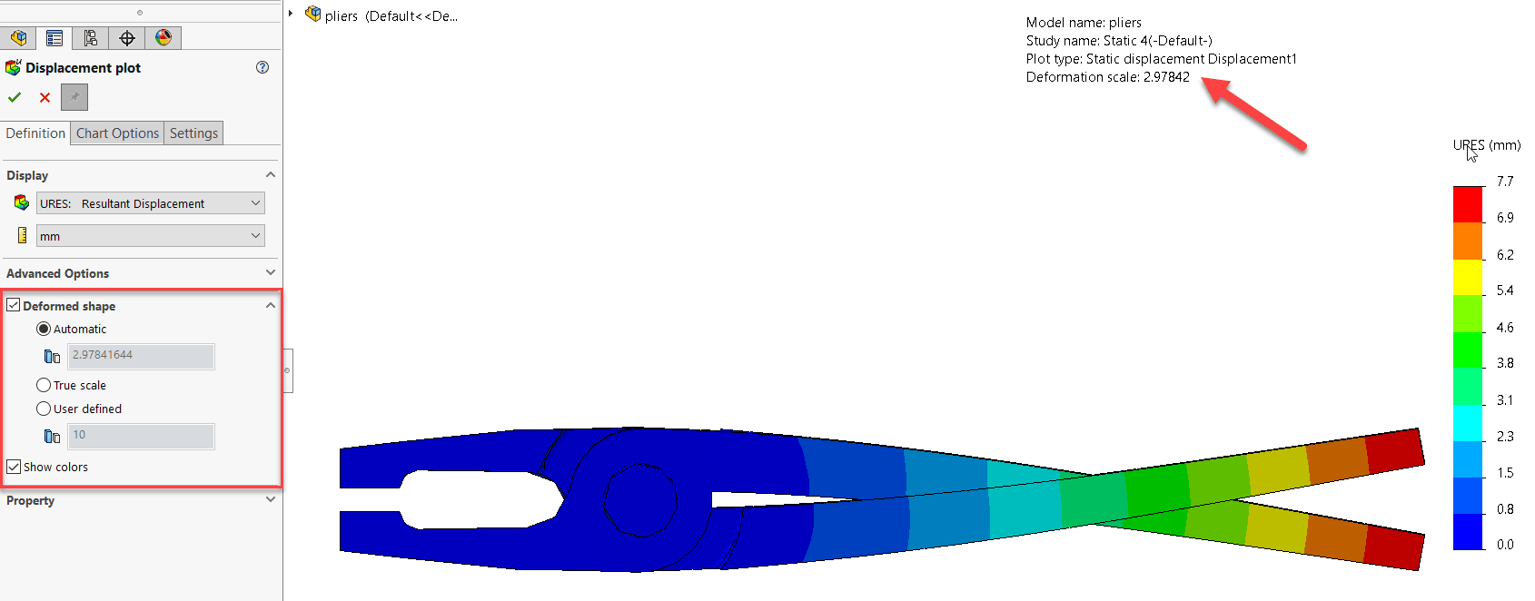
Figure 2: Strange looking results with Automatic deformed shape scale factor

In this particular case, I’d want to set the deformed shape scale factor to “True scale”, which shows the tips of the handles contacting one another correctly.

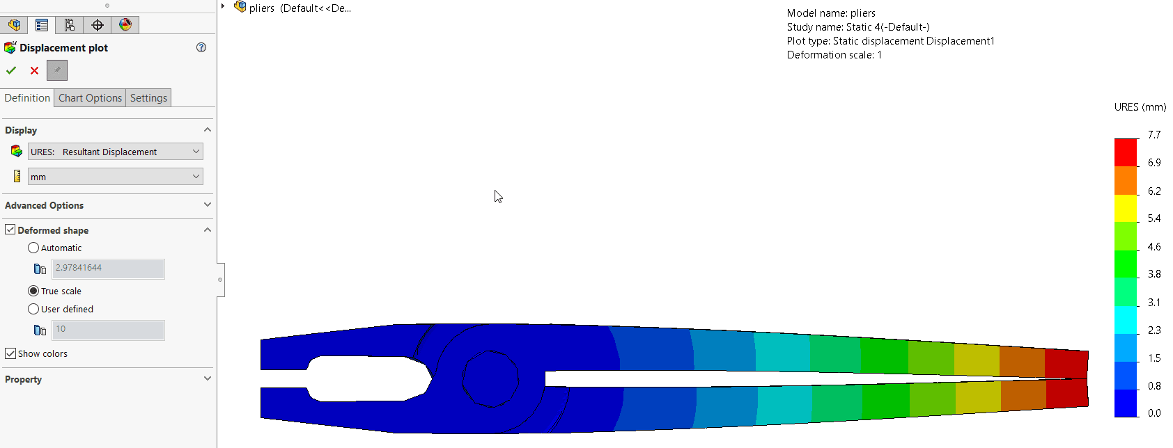
Figure 3: Expected results with True scale factor applied

The next step is to animate the displacement plot. Right click on the displacement plot in the results folder and selecting animate.

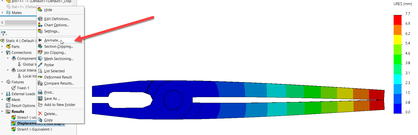
Figure 4: How to animate your displacement plot

Once the animation property manager displays, hit the play button and observe how your model deforms and deflects under the applied loads, fixtures and interactions. Most designers and engineers have a good intuition for how their parts and assemblies will deform. A displacement animation is a helpful way to confirm that your instincts are correct (or perhaps not).

If your study passes these deformation sanity checks, you can now proceed to post-processing of the stress results.

Tip #2: Use “Discrete” instead of “Continuous” for contour plots

When analyzing your stress or deformation results consider switching the contour display from “Continuous” to “Discrete”. Right click over the legend and then select “Fringe Options” and then “Discrete”.

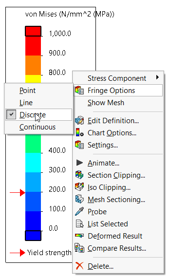
Figure 5: How to switch from “Continuous” to “Discrete” contour display

“Continuous” will blend and blur together the colors in the legend as shown in the image below.

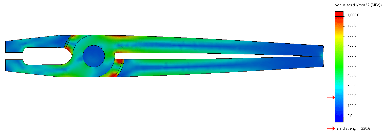
Figure 6: “Continuous” von Mises stress

“Discrete” will create more distinct color bands to delineate differences in stress or deflection in your plot as shown in the image below.

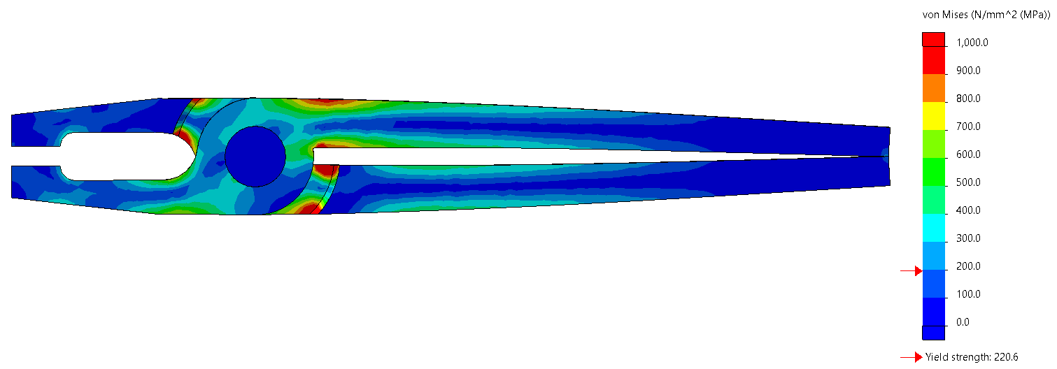
Figure 7: “Discrete” von Mises stress

Whether to use “Discrete” or “Continuous” is a personal preference, but I find the discrete option better for post processing contour plots.

Tip #3: Reset both the upper and lower bounds of your legend

When plotting stress results, the default upper limit shown on the legend will be the maximum stress in your model. Similarly, the default lower stress limit will be the minimum stress in the model.

The maximum stress in the model is often a local “hot spot” associated with a fixture or area of high contact stress. This will often leave a “sea of blue” in the rest of the model indicating stresses that are low relative to the maximum in the model, as demonstrated in the image below. However, the blue and green colors may actually be high stresses relative to the strength of the material.

Figure 8: Default upper and lower bounds for von Mises stress

We know that stresses near fixtures are not accurate and must be considered with skepticism or ignored. So why set the upper bound of the color legend on the maximum (likely inaccurate) stress result near a fixture or hot spot?

Instead, experiment with adjusting the upper and lower bounds for more insight into the stresses in your model and to eliminate the “sea of blue”. Left click on the upper or lower bound number of your legend and key in different numbers. In the example below I chose 500 MPa as my upper limit. I also changed the lower limit from the default 1.6 MPa to 0 MPa.

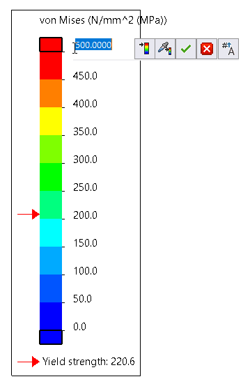
Figure 9: Changing the upper bound of von Mises stress

These changes create round number increments of exactly 50 MPa for each color band. If I had left the lower bound at 1.6 MPa, this would not have been in the case, because it divides the color bands evenly between upper and lower bounds. Having the lower bound be exactly 0 MPa makes logical sense. Note that in the image below we now see much more orange, yellow and green which are areas of high stress, far in excess of the yield strength of the material, indicating that a design change is necessary on this model. This was less obvious with the default bounds on the stress plots.

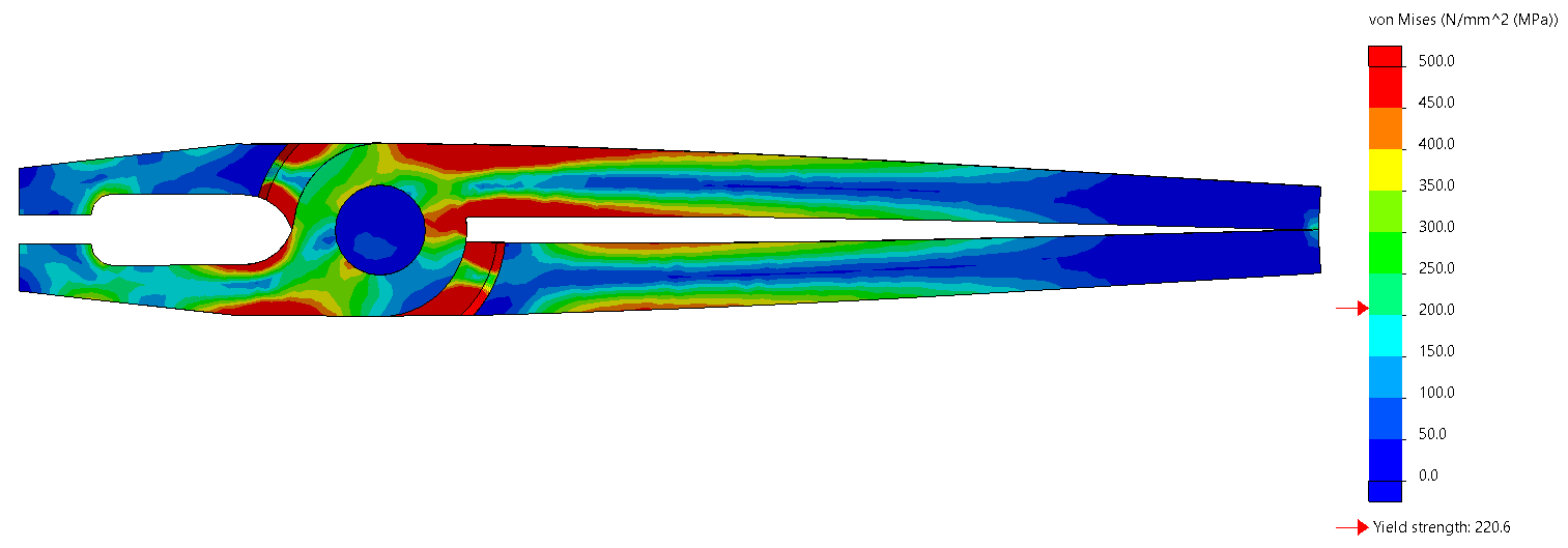
Figure 10: Modified upper and lower bounds for von Mises stress

There are lots of other useful tricks for post processing in SOLIDWORKS Simulation but I hope these tips will be useful and improve your understanding of the results. Now go design some innovative products with the help of SOLIDWORKS Simulation.

Alon Finkelstein
Simulation Product Specialist
Computer Aided Technology, Inc.