SOLIDWORKS Simulation: Calculating Convection and Verifying Thermal Results

I have been asked a few times about calculating and applying a convection boundary condition for SOLIDWORKS Simulation Thermal analyses, because without a CFD software, like SOLIDWORKS Flow Simulation, convection must be calculated by hand. As you may already know, there are three modes of heat transfer; conduction, convection, and radiation. SOLIDWORKS Simulation will calculate conduction, but it is up to us to define the parameters for convection and radiation. In this blog I will calculate the convection coefficient of a horizontal copper pipe, simulate the temperature distributions of the pipe using a Thermal study, and verify the results using SOLIDWORKS Flow Simulation.

Convection is simply conduction from a solid to a fluid. They both obey Fourier’s Law;

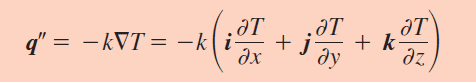
Equation 1: Fourier’s Law

but instead of using the material property, thermal conductivity, this constant depends on many variables that define the boundary layer of the fluid, which is why Equation 1: Fourier’s Law can be simplified to Equation 2: Newton’s Law of Cooling.

Equation 2: Newton’s Law of Cooling

The convection coefficient, formally denoted by h, is what is needed for our thermal analysis in SOLIDWORKS Simulation. In this thermal analysis we have a long hollow copper pipe (20 mm OD and 15 mm ID) that is transporting a hot fluid (80 C) through a body of water (20 C). We will also assume the body of water is static and, therefore, the convection is defined as natural rather than forced convection.

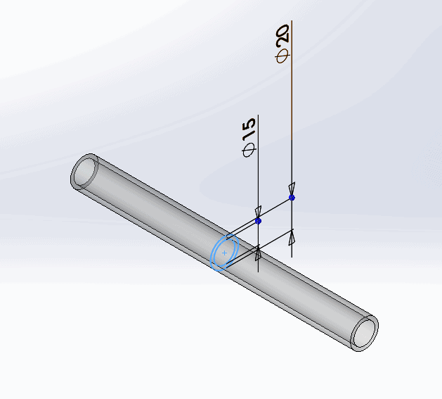
To keep things simple, we will assume that the inner surface of the piping will remain constant at 80 C and only simulate a 200 mm section of the length since the results will remain constant in the axial direction. The first step in calculating h is to determine if the boundary layer of the fluid is laminar or turbulent, because the boundary layer is the main contributor to the effectiveness of convective heat transfer. It is customary to quantify the boundary layer using the Rayleigh number (Ra).

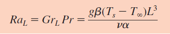
Equation 3: The Rayleigh Number

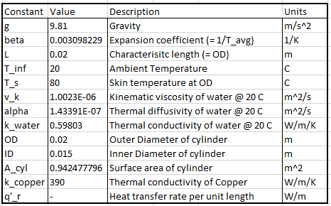
Where v and α are the kinematic viscosity and thermal diffusivity of the fluid respectively. Most textbooks will say that fluid properties should be looked-up and/or calculated at an average temperature (skin temperature and ambient temperature), but in my experience it is more accurate to look-up fluid properties at T_∞ (= 20 C). Ra for my copper pipe, where T_s = 80 C, T_∞ = 20 C, and L = OD = 0.02 [m], was calculated as

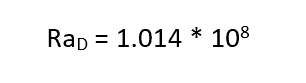
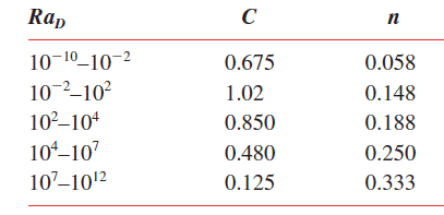
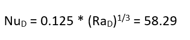
Once calculated, Ra is then used to determine which equation is appropriate for calculating the average Nusselt number (Nu) (because of space restrictions a complete list of variable definitions can be found in the table at the end of this blog).

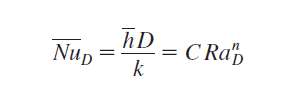
Equation 4: The Nusselt Number for Long Cylinders

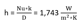
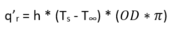
And, finally, the average convection coefficient, h, can be calculated directly with Nu by rearranging Equation 4 to solve for h.

But wait! We are not quite ready to put this number into our thermal analysis. We are assuming that the ID of the pipe remains constant at 80 C, but the OD is the surface that is transferring heat to the fluid. We need the surface temperature of the OD to calculate a more accurate h. Luckily, we can estimate it by assuming the same amount of heat, q_r, will travel through the pipe since it has a 2.5 [mm] wall thickness and Copper has such a high thermal conductivity.

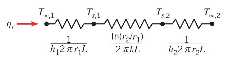
Equation 5: Thermal Resistance of a Pipe

This yields

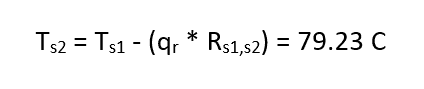
where

Now, if you are like me and created an Excel spreadsheet to perform your calculations it will be easier to calculate the new h at T_s = 74.2 C. Make sure your new Ra does not affect the Nu = f(Ra) relationship since the constants, C and n, for the exponential relationship are dependent on Ra, which will remain the same in this case.

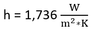
As you may have noticed, our new h is approximately the same as the original h, which means our assumption that q_r remains approximately equal was valid. But, it is always good to do a gut check.

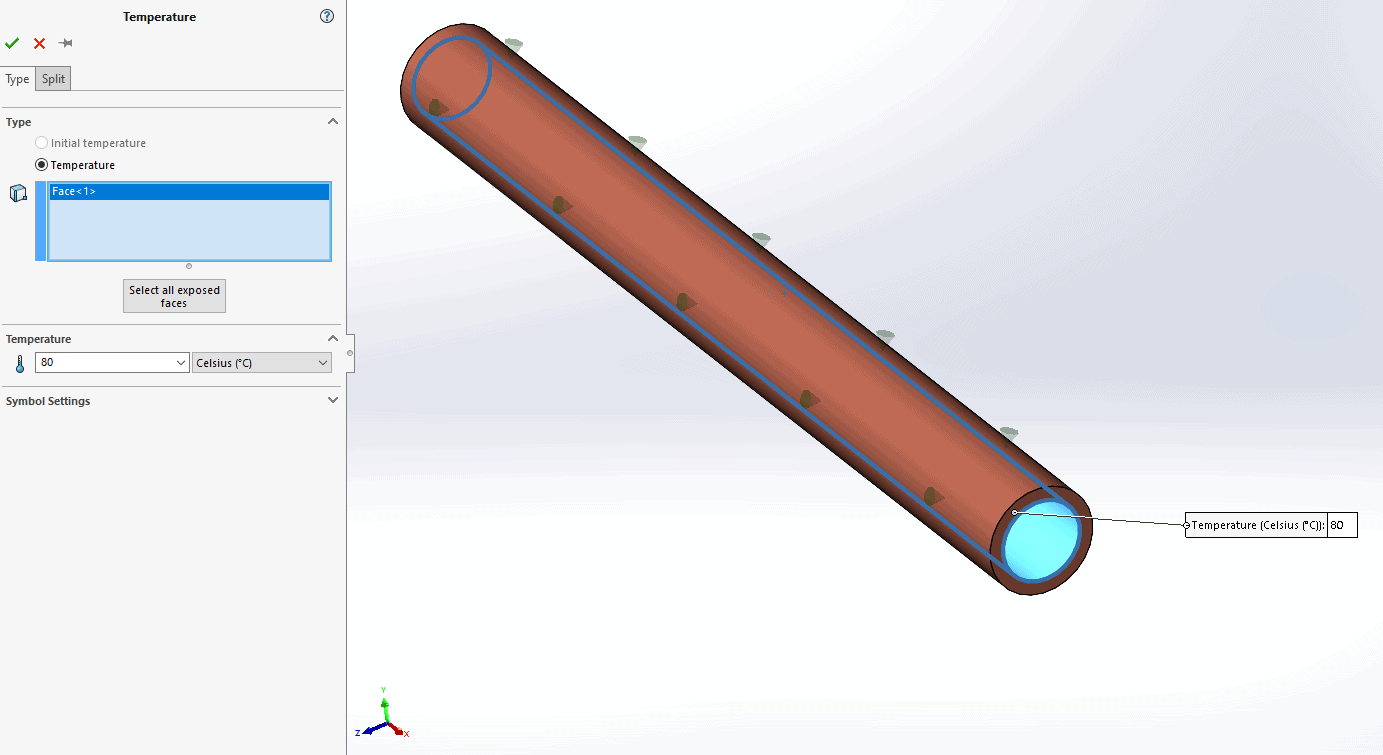
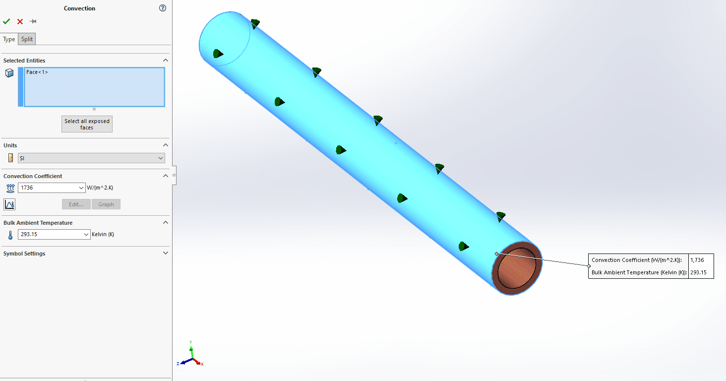
Now, we are ready to setup the thermal study. Once the material is applied and the study properties are set, we define the ID as 80 C and apply our new h to the outer surface.

Finally, we are ready to run the thermal analysis once the mesh is sufficiently refined.

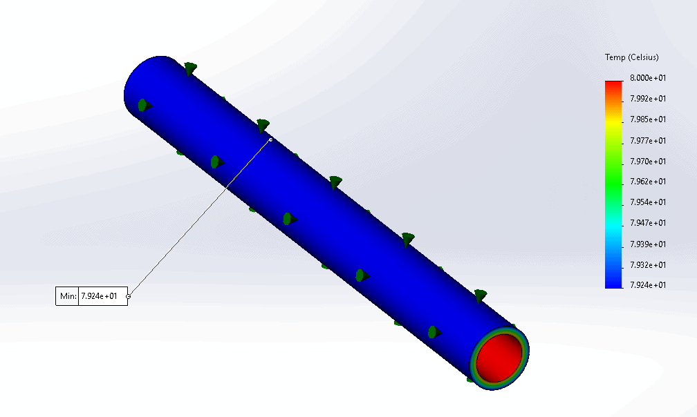
With a surface temperature of 79.24 C at the OD, which closely matches our original prediction of 79.23 C, we are now ready to verify our SOLIDWORKS Simulation results with SOLIDWORKS Flow Simulation.

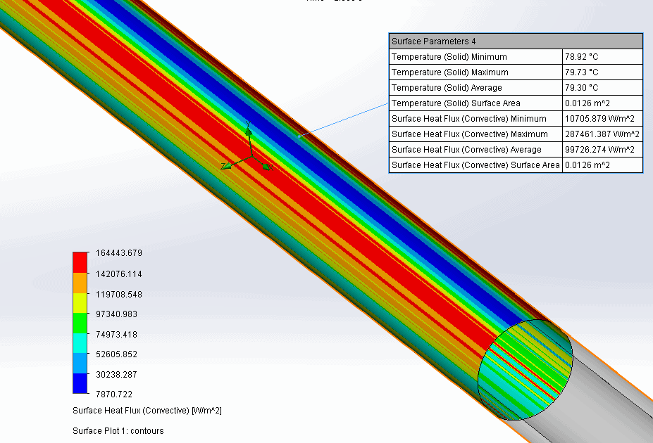
Comparing the results, we can see that the average temperature and heat flux are agreeable, which means we can trust hand calculations after all!

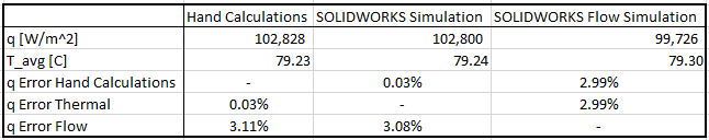
The main reason why CFD software is needed becomes apparent after seeing the differences in SOLIDWORKS Simulation temperature plots and the surface heat flux plot with SOLIDWORKS Flow Simulation. Our thermal analysis has no gradient across the outer surface while the CFD result plot is much more detailed, which is precisely the reason why applying a convection boundary condition in a thermal analysis is an averaged approximation and should only be used for global trends. With this in mind, the time that can be saved using SOLIDWORKS Simulation exponentially increases as model geometry increases in complexity!

While the known correlations for Nu and various geometry are limited to simple shapes (flat plates, cylinders, spheres, etc.), there is always a way to make more assumptions and calculate the convection coefficient so SOLIDWORKS Simulation can be utilized.

Cameron Bennethum
Support Engineer – Simulation
Computer Aided Technology, LLC