What’s the Difference Between C3D10 and C3D10HS Elements?

And When Do You Use One Over the Other?

The C3D10 and C3D10HS are both 10 node tetrahedral elements in Abaqus with quadratic interpolation of displacement, otherwise colloquially referred to as “2nd order tets”. While the C3D10 is the standard or “vanilla” 2nd order tet element, C3D10HS is marketed as a 2nd order tet element with improved surface stress visualization. To understand how and why C3D10HS is different from C3D10, we need to quickly review how stress is calculated using the Finite Element Method (FEM) and how stress is visualized on the mesh using a contour plot.

Some Background: How Abaqus Calculates Stresses

First, on visualization, for Abaqus to create a contour plot of any variable, it requires the values of that variable on individual nodes which it then uses to assign colors to different regions of the mesh. So, to create a contour plot of stress, Abaqus needs the stress values at individual nodes. The issue with this is that stress values are not calculated at the nodes, which brings us to the point of how stress is computed using FEM.

Without going too much into the details, users must know that displacement is the first quantity computed using FEM as it currently exists. This displacement is calculated at the nodes, and therefore Abaqus can easily create contour plots of displacement without the need for a special “improved surface displacement” element. Other nodal quantities are forces of any kind (for e.g., reaction forces) and temperature. To calculate stress from this displacement, the software first needs to compute the strain.

This calculation of strain from displacement involves differentiation. Common computers, in their current form, are either incapable or very inefficient in performing analytical differentiation, and thus, differentiation in software like Abaqus is “pre-coded” and calculated at integration points only. This implies that strain in an element is only available at the integration points which are located below the surface of C3D10 elements (see Figure 1). This strain is then combined with the material data provided by the user to compute the stress, again at the integration points.

The Problem Arises: Issues of Extrapolation

However, for creating a contour plot, this stress needs to be extrapolated so that stress at nodes are obtained and a contour plot is created. This extrapolation process for the purpose of creating the contour plot, unfortunately, is completely numerical, is performed without regard to the material properties of the element. This can sometimes cause some nodal stresses to have un-realistic values (e.g., being more than ultimate tensile stress of the material). This extrapolation is especially egregious in badly shaped elements as even small differences in integration point values of stress can get magnified when extrapolated to the nodes.

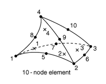
Figure 1: Position of nodes and integration points (x) in a C3D10 element. There are 4 integration points and 10 nodes. Extrapolation can lead to misleading contour plots, especially for badly shaped elements.

The Solution: C3D10HS

The C3D10HS element overcomes this “curse of extrapolation” by having the integration points co-located with the nodes, so that no extrapolation is required for creating contour plots of strain and stress values. This brings the number of integration points in a C3D10HS element up to 11 (10 points co-located with the nodes and one at the element centroid) instead of 4 for C3D10. As a result, they give a better estimate of the stress when stress is read off of the color contours.

C3D10HS elements also engage a hybrid solution for stress based on internal pressure (in addition to displacement), when the material exhibits behavior approaching the incompressible limit (i.e., an effective Poisson’s ratio above .45). This unique feature make C3D10HS elements especially suitable for modeling metal plasticity, since the feature activates only in the regions of the model where the material is incompressible.

When to Use Which: C3D10 vs. C3D10HS

Figure 2: The correct stress value in the fillet is 200 MPa (based on Peterson’s Stress Concentration Factors). C3D10HS fine, C3D10 fine, C3D10HS coarse, and C3D10 coarse mesh, respectively, show the same results.



Figure 3: As the stress begins to exceed yield (300 MPa), faulty extrapolation (dark red) becomes apparent in the C3D10 elements. Download this model to test for yourself.

C3D10HS elements provide superior stress visualization, especially in coarse meshes, as they avoid inaccuracies due to stress extrapolation. This is generally nice to have, but especially so when presenting stress results to individuals who are unfamiliar with FEA. C3D10HS elements also exhibit improved convergence under incompressible material conditions, making them a better choice when modeling metal plasticity or other incompressible materials.

Both of these benefits come with increased computational cost, so that is the trade-off you must consider. For brick meshers, there is a version for you, too, aptly named C3D8HS. These elements are available in Abaqus/Standard only, and you may wish to output stress at only the nodes in order to reduce ODB size.