SOLIDWORKS Simulation: Boundary Conditions and Linear Thermal Expansion (Part 1)
I’m sure you’ve heard the saying “garbage in, garbage out”. This applies to lots of things we encounter in life, including our analysis work. What if you didn’t realize your input was faulty until you review your analysis results and find garbage out? Would you be able to backtrack your steps and find where you made a mistake? What if it wasn’t really a mistake, but a misunderstanding as to how a specific tool operates? I’m going to show you an example of this by using temperature boundary conditions and linear thermal expansion with SOLIDWORKS Simulation.
The model I’m going to work with is a 20 mm per side cube subjected to a 100 C temperature increase. I’m going to use a 1/8th symmetric model for the analysis. This allows me to use three symmetry restraints on the inside cut faces. This fixture scheme permits the cube to expand or contract as if the center of the cube were fixed and will not adversely affect the displacement results. The orange arrows in Figure 1 indicate the faces that will have a Symmetry restraint applied.
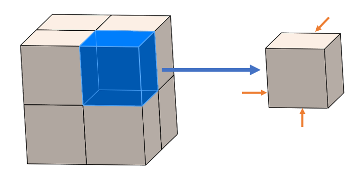
Figure 1
With the 1/8th symmetric cube built and saved, I created a new Linear Static study with SOLIDWORKS Simulation. I added the three symmetry restraints previously discussed. Then I assigned a custom material based upon annealed, stainless steel bar stock; material properties shown in Figure 2. For temperature boundary conditions, the important material property is the Coefficient of Thermal Expansion.
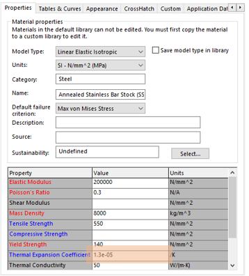
Figure 2
Next, I’ll review the properties of the Linear Static study, specifically the Flow/Thermal Effects tab and review the setting for Reference temperature at zero strain, set to 25 C (Figure 3).
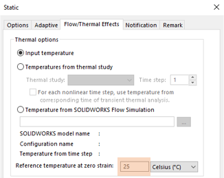
Figure 3
The last boundary condition that I want to add is a temperature to the entire body of the cube, 125 C. I’ll cover the boundary conditions shortly, but at this point I could use a hand calculation to solve for the linear thermal expansion of the cube (Figure 4). The length along any edge is 100 mm and the change in temperature is 100 C.
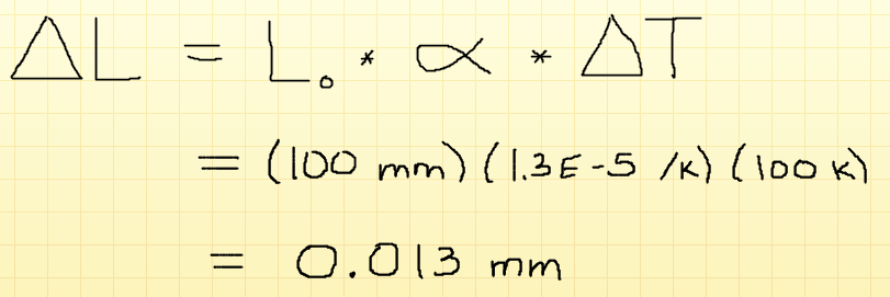
Figure 4
Now I know that I should obtain a directional displacement (Ux, Uy, or Uz) equal to 0.013 mm from the linear static study.
Now let’s look at garbage in, or how not to apply the temperature boundary condition. I want to add the 125 C temperature to the cube, so I right-click on the External Loads folder and select Temperature. When the Temperature property manager appears, uninformed SOLIDWORKS Simulation users often click the Select all exposed faces button to apply the thermal boundary condition to the finite element model (Figure 5).
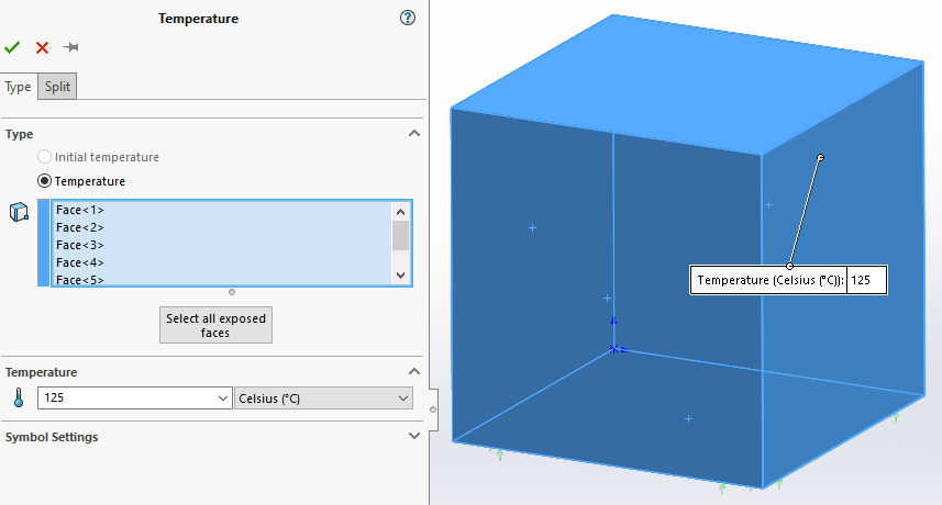
Figure 5
After adding the thermal load, I meshed and solved the linear static study. The result I am interested in is resultant displacement followed by any of the three directional displacements. The resultant displacement plot is shown in Figure 6.
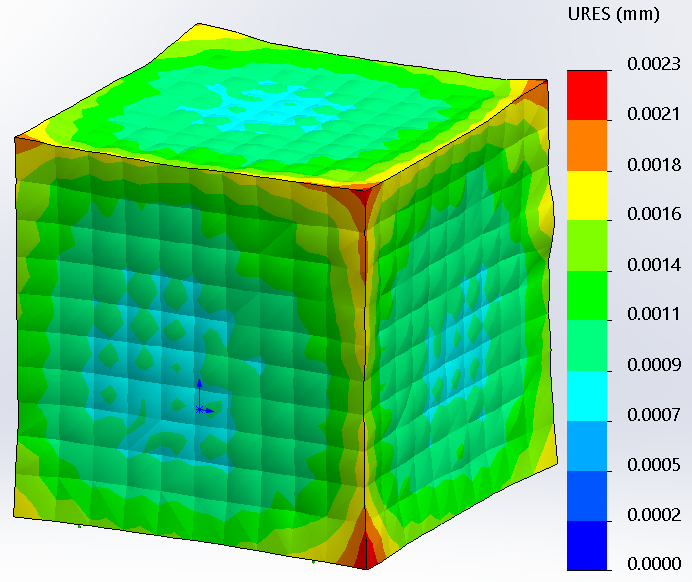
Figure 6
As soon as I see this result, I know that I have garbage out. What I should have obtained is the cube uniformly expanding in the positive X, Y, and Z directions from the origin of this 1/8th symmetric model. The result appears to have expanded the cube in some regions but contracted it in others.
The mistake in the boundary condition, as pointed out earlier, was the use of ‘Select all exposed faces’. At first glance, you might think that the three cut faces of the model with the symmetry restraints should not have had the temperature applied. That might be correct if the finite element analysis were a Thermal study and not a Linear Static study, but that isn’t the case here. What I should have done is applied the temperature boundary condition to the entire body. To accomplish this, I should have utilized the Flyout Feature Manage Design Tree (hit the C key on your keyboard if you don’t see it), then expand the Solid Bodies folder and select the body to assign the temperature (Figure 7).
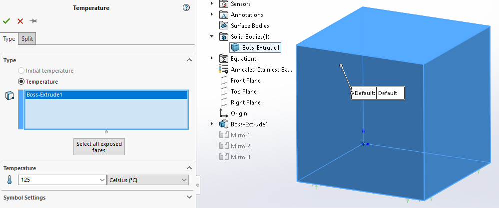
Figure 7
After correcting the temperature boundary condition, I re-calculated the FEA study and obtain the results shown in Figure 8. The resultant displacement clearly shows a uniform expansion along all three axes on the left side of the figure. The right side shows a Z-displacement equal to 0.013 mm, matching the hand calculation shown in Figure 4.
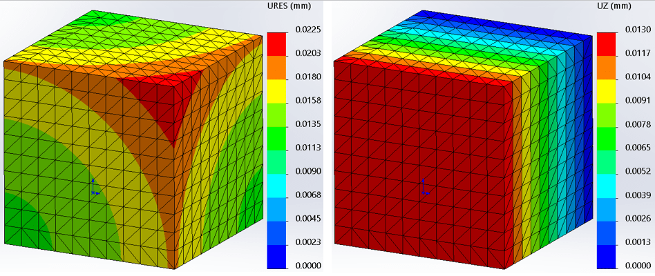
Figure 8
There are a few things to note about what you’ve read here. I did indicate that the initial temperature boundary condition was incorrect before I reviewed the results – garbage in. If only the rest of our analysis work were so simple that someone would tell you what you did was wrong before you go down a long path to find garbage out! In this example, as well as any analysis work you do, I think it’s incredibly important to have an idea of what the results should be prior to jumping into a computer simulation. Perform a hand calculation first, if you can. If not, at least start with a simplified version of your CAD model and work through a few iterations of preliminary analysis studies before you dig into a large and involved computer model. If you do that, you will gain in understanding how the full digital clone might perform . I’ve written about this in some of my other blogs and I know the rest of my Simulation Team counterparts would agree! As to the “why” the garbage out resultant displacement occurred, as shown in Figure 6, I will explain that in Part 2 of this blog. Now go make your products better with SOLIDWORKS Simulation!

Bill Reuss
Product Specialist, Simulation
Father, golf junkie, coffee connoisseur, computer nerd
Computer Aided Technology, LLC