SOLIDWORKS 2018 What’s New – Flow Simulation Noise Prediction – #SW2018
SOLIDWORKS 2018 What’s New – Flow Simulation Noise Prediction – #SW2018
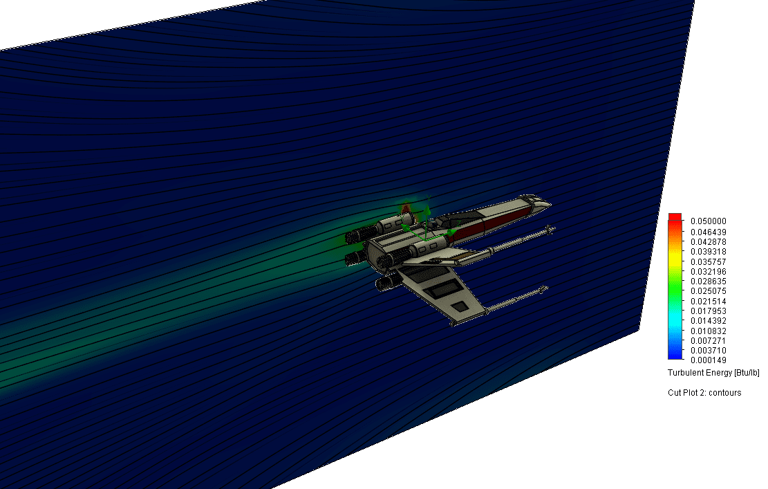
For many engineer’s noise intensity due to flow turbulence is a critical design criterion. Designers must consider noise output from industries as diverse as kitchen appliances, automotive, and defense. Unfortunately, not until recently, users could only interpolate a general sense of noise output by viewing turbulence plots.
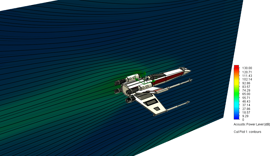
Now, in SOLIDWORKS 2018, Flow simulation has new capabilities to show acoustic plots. The image below utilizes decibel (dB) units to display acoustic power.
How is Acoustic Power determined?
Proudman, using Lighthill’s acoustic analogy, derived a formula for acoustic power. This formula was rederived by Lilley to account for the retarded time difference which was neglected in Proudman’s derivation. These formulas provide acoustic power due to unit volume of isotropic turbulence (in W/m3).
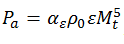
Where Mt is the turbulent Mach number; αε is a model constant equal to 0.1, based on the calibration of Sarkar and Hussaini; ρ0 is the density of the medium, ε is the turbulent eddy dissipation. A log function is used to transform the solution into decibel (dB) values.
Interpreting results.
Sound ranges, in the decibel domain, between 0 and 194. This range is subject to atmospheric conditions. In the interest of providing perspective; a normal conversation would be roughly 55 dB, a chainsaw runs at 100 dB, and a jet engine would register at 150 dB.
Noise prediction is limited to the broadband noise characteristics prediction and does not provide any tonal performance data. Also, one should be aware of the assumptions made in the derivation. These assumptions are as follows; high Reynolds number, small Mach number, isotropy of turbulence, and zero mean motion
I hope this part of the What’s New series gives you a better understanding of the new features and functions of SOLIDWORKS 2018. Please check back to the CATI Blog as the CATI Application Engineers will continue to break down many of the new items in SOLIDWORKS 2018. These articles will be stored in the category of “SOLIDWORKS What’s New.” You can also learn more about SOLIDWORKS 2018 by clicking on the image below to register for one of CATI’s Design Innovation Summits.
Matthew Fetke
Application Engineer