Recommendations to Achieve Accurate Results with Linear Dynamic Analysis

Our Simulation team gets asked a lot of questions regarding SOLIDWORKS Simulation features, capabilities, how-to, and similar, by our Simulation users.  After answering this myriad of questions, the most common theme for a follow-up is almost always related to achieving accurate results with SOLIDWORKS Simulation.  Our Simulation team has written several blogs that provide guidance related to meshing and accuracy, such as Take Control of Your Mesh, Nodal vs Elemental Stress, one of my long-time favorites Divergence and Convergence for Simulation Results, and How Accurate are Your Results.  Yes, the accuracy of analysis results is a kind of a big deal!  While each of these articles are valid for all types of analysis work, some types of structural analysis require a few additional steps.  Linear Dynamic analysis in SOLIDWORKS Simulation Premium is one such example.  To achieve valid results using Linear Dynamic analysis in SOLIDWORKS Simulation Premium, you first need to have an understanding as to how this type of problem is solved.

Let’s start with the basics.  Linear Dynamic analysis in SOLIDWORKS Simulation Premium follows three general guidelines.

• Material properties remain constant, elastic for all loading conditions.
• Displacement results are small compared to the original geometry.
• Time-dependent loading conditions.

It’s the details of this third requirement that add work to successfully solve Linear Dynamic studies with SOLIDWORKS Simulation Premium.  The solution technique is called ‘Modal Superposition’.  This technique allows us to solve problems like shock and impact loads, simulate shaker table tests, or even analyze seismic loading conditions.

You can search for the definition of superposition and come up with several lengthy descriptions for what it means.  The best description I’ve read can be summed up (pun intended) as “for an independent number of influences acting on a linear system, the resultant is related to the sum of the individual influences acting separately”.  Modal Superposition, and thus all Linear Dynamic analyses, start with analyzing the resonant frequencies of the structure to extract the eigenmodes.  The eigenmodes are used for building the summation of the individual linear system influences to generate the full solution.  I think this concept is best described visually!

Let’s start with a structure that has the first six natural frequencies, shown overlapping on a single chart (Figure 1).  (This output looks an awful lot like what you could achieve with a Spirograph when you were a kid!  Does that show my age?)

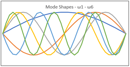
Figure 1

Utilizing a ‘Natural Frequency’ study, the analysis extracts the individual eigenmodes (Figure 2).  (Specifying the number of natural frequencies to solve for is an option in the Study Properties of Natural Frequency analysis as well as Linear Dynamic analysis.)

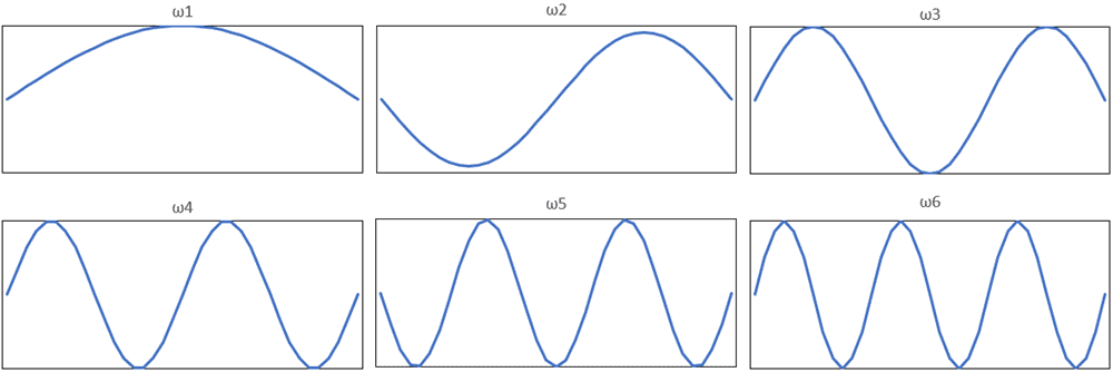
Figure 2

The next step in the solution process is to analyze the system response from each input for each eigenmode, then sum the results together.

Let’s first consider a simple example where only the first two modes are included and the frequency of a single input is near the second natural frequency, ω2.  If the input causes a response at each of the included modes, the full response of the linear system can be approximated by the summation of modes 1 and 2.  The response to this scenario is shown in Figure 3.

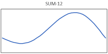
Figure 3

What if the frequency of the input was closer to the frequency of ω6 and it generated a response at each of the first six modes?  If the number of frequencies included in the Linear Dynamic study was limited to the first two modes, the response can only follow what is shown in Figure 3.  By limiting the number of modes included in the analysis, the response of the system and, thus, the results of the analysis are incorrect!  This would hold true for any Linear Dynamic analysis where only the first three, four, or five modes are included in the analysis.  It’s not until at least the first six modes are included in the Linear Dynamic study that the correct response can be achieved.  Reference Figure 4 to visualize how the summation of the individual modes could potentially affect the results.

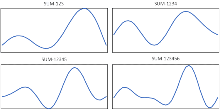
Figure 4

Hopefully, that visually explains how Modal Superposition is used to solve Linear Dynamic studies.  Now that you’re armed with a basic understanding of Modal Superposition, how can we use this to achieve accurate results from our Linear Dynamic analysis work?  Quite simply we need to add additional guidelines to the first three previously mentioned.

One additional guideline builds upon what I previously described in how Modal Superposition functions.  You need to verify that the highest included mode is significantly larger than the highest input frequency.  Once you have solved the Frequency analysis for a Linear Dynamic study, right-click on the Results folder and choose ‘List Resonant Frequencies’ (Figure 5).  Scroll to the bottom of the list and verify the frequency of the highest included mode.  Depending upon the source, you may find guidance that the highest included mode be at least twice the maximum input frequency, though I’ve also read this should be 5x higher.  I think it’s safe to start with 2x and increase, as necessary.

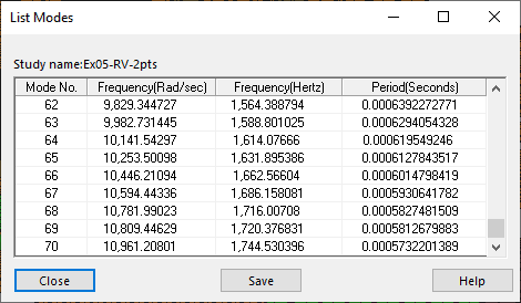
Figure 5

Another additional guideline is to verify the Mass Participation for the number of included modes.  You can verify this with a right-click on the Results folder and choosing ‘List Mass Participation’ (Figure 6).  Scroll to the bottom of the list and review the sum of mass participation for the included modes in the X, Y, and Z direction.

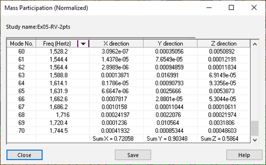
Figure 6

Alternately, you could create a Frequency Response Graph to create a Cumulative Effective Mass Participation Factor (CEMPF) plot for a better visual of this data (Figure 7).  In general, you would like to have greater than 80% of the structures’ mass included with all modes of the study.  For some finite element models, this is impractical as it could require thousands of modes be included in the analysis.  In this case, check to see that you have greater than 80% CEMPF in the direction of the time-based input, as a start.

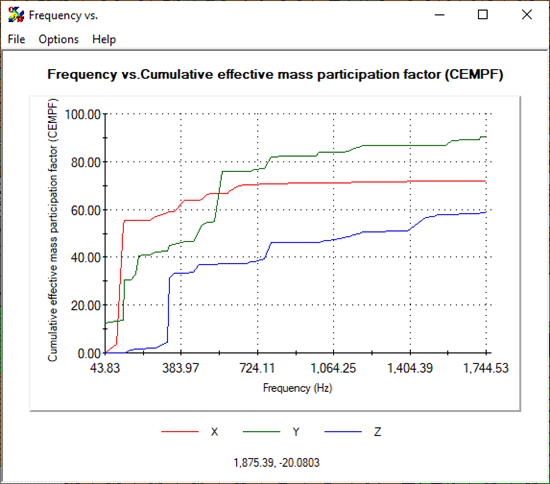
Figure 7

Now solve your Linear Dynamic study and review your results!  But how accurate are those results?  The way to verify accuracy takes a few steps.  You can follow a mesh convergence process to verify regions of high stress, which is common for Linear Static studies.  For Linear Dynamic studies, you should also increase the number of modes included in the analysis by ~10% (or more) and re-solve the study to verify the results do not significantly change.  You may need to increase the number of modes a few times to verify convergence.  Now go make your products better with SOLIDWORKS Simulation!

Bill Reuss
Product Specialist, Simulation
Father, golf junkie, coffee connoisseur, computer nerd
Computer Aided Technology, LLC