SOLIDWORKS Flow Simulation: Lift Up Your Design
SOLIDWORKS Flow Simulation: Lift Up Your Design
If you have ever done any aerodynamic testing, you know that wind tunnels (or time in one) are expensive and requires a lot of pre-testing setup and a lot of data gathering. After running the tests all day, next comes the arduous task of data analysis from the limited data you have collected. SOLIDWORKS Flow Simulation can help reduce the time and effort required to gather data about a potential aerodynamics problem. To demonstrate this, I have taken advantage of some of the features available in Solidworks and Flow Simulation.
The first task is to get the airfoil shape into the SOLIDWORKS environment. This can be accomplished by importing a curve generated from an airfoil profile plot. For this particular example, we will be using a NACA 4412 airfoil profile. As the parametric math governing the airfoil shape is rather complex, it is often much faster to use a plotter that can output a series of XY points that define the curve. For Solidworks to import this data, it needs to be an XYZ data set that is tab delimited. This is a standard output formula in Excel and other plotting software.
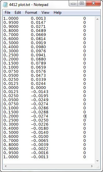
From this point, one can import these points into a curve in the Solidworks environment using the Curve through XYZ points and import the .txt file into Solidworks.
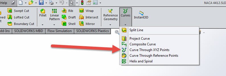
This will generate a continuous curve through the points listed in the file.
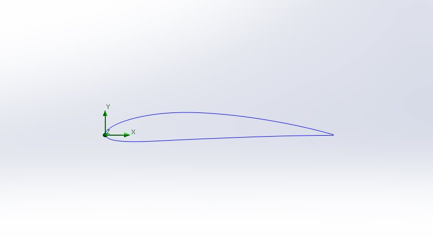
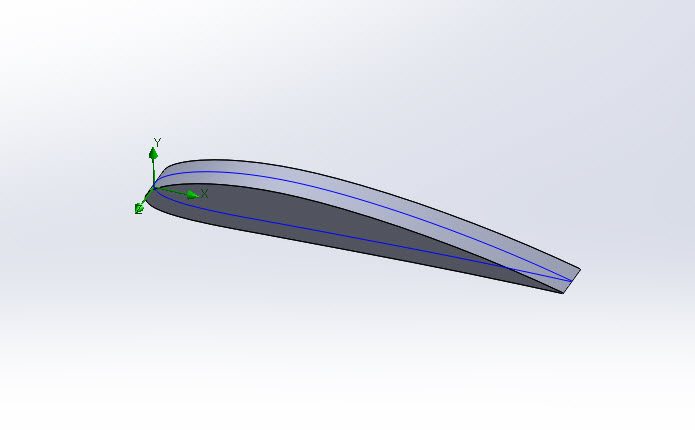
After that, start a new sketch on the plane parallel to the imported curve and use the convert entities tool to make that curve into a sketch entity. After the sketch is verified as a closed contour (you may have to add a small final sketch segment to close the profile), one can use the extrude command to create a small wing section.
Once the wing has been built, one can start the flow simulation and begin defining the problem. To start, we will be doing an external simulation with air as our fluid medium. When we get to the initial conditions, we will be using the aerodynamic angles version of the velocity definition.
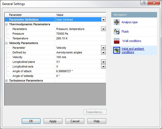
This allows us to define the flow direction with respect to an angle of attack on the airfoil. For this example, we are simulating flying at 3000m above sea level (ASL) so the pressure is 70,000 Pa and the air is at a chilly -5 C. We will be traveling at 195 knots or 100 m/s. Since we are testing a prismatic airfoil shape, we can make use of the 2D simplification in order to reduce the computational load.

Now that we have our computational domain and our settings complete, we need to create some goals in order to evaluate our airfoil. We start with some pressures and velocities to keep our convergence tight. Then we also utilize the force in the x and y directions. These will subsequently be used to create our co-efficient of lift and drag goals. In order to calculate these values, we need to have a few pieces of data on hand. We need to know the fluid density, the velocity, the force normal and parallel to the fluid flow, and the planform (projected) area of the wing profile. Because the angle of attack changes relative to the coordinate axis, we need to use trigonometric relations to get the forces with respect to the fluid direction defined by the angle of attack (alpha).

These values are entered into the equation goals and will be evaluated as the solver progresses. Included are the reference equations.
![]() (Drag Coefficient)
(Drag Coefficient)
![]() (Lift Coefficient)
(Lift Coefficient)
Fd= Drag force L=Lift Force ρ=Density ν= Velocity A & S=Planform Area
From this point we need create a parametric study that will vary the angle of attack across several studies. We also want to include several cut plots and an x-y plot that is generated by the curve that defined the airfoil profile. Also needed are all the relevant goals.
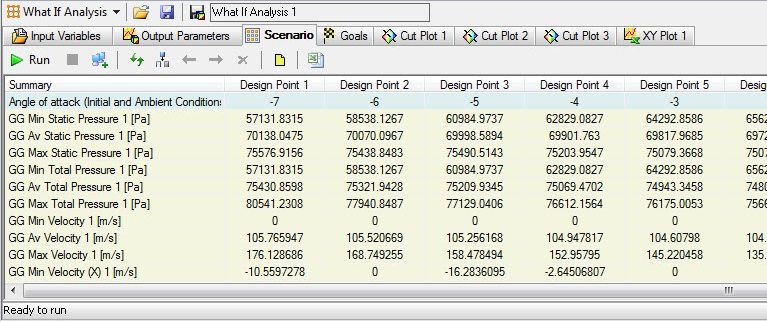
Once the study has run its course through all the angles of attack, one can plot the results and compare them with theoretical charts to show that the solver worked well for this study. The results are compared with an inviscid solver (Xfoil) that makes several assumptions that the flow solver does not. Notice how the solver captures the effects of the airfoil much more accurately and does not “neatly” follow the theoretical curve. This is much more like real wind tunnel data once the appropriate corrections to the tare and force sensors are made. The comparisons are shown below. Note that the Cd and CL were calculated with a Reynolds number of ~1,000,000 while the size of the airfoil in use makes the solver Reynolds number ~15,000,000. This makes the scale of the drag slightly different but the trends remain.


As you can see, SOLIDWORKS Flow Simulation can be used very effectively to simulate airfoil design parameters and can easily shave time and money off of your design process by reducing expensive wind tunnel or flow bench testing time while giving far more confidence in the design iteration process.
Blog Post By: Drew Potter